We wrap up the discussion on partitioning from our collective favorite book, Designing Data-Intensive Applications, while Allen is properly substituted, Michael can’t stop thinking about Kafka, and Joe doesn’t live in the real sunshine state.

The full show notes for this episode are available at https://www.codingblocks.net/episode172.

Sponsors

• Datadog – Sign up today for a free 14 day trial and get a free Datadog t-shirt after creating your first dashboard.
• Linode – Sign up for $100 in free credit and simplify your infrastructure with Linode’s Linux virtual machines.

Survey Says

News

• Game Ja Ja Ja Jam is coming up, sign up is open now! (itch.io)
• Joe finished the Create With Code Unity Course (learn.unity.com)
• New MacBook Pro Review, notch be darned!

Last Episode …

Best book evar!

In our previous episode, we talked about data partitioning, which refers to how you can split up data sets, which is great when you have data that’s too big to fit on a single machine, or you have special performance requirements. We talked about two different partitioning strategies: key ranges which works best with homogenous, well-balanced keys, and also hashing which provides a much more even distribution that helps avoid hot-spotting.

This episode we’re continuing the discussion, talking about secondary indexes, rebalancing, and routing.

Partitioning, Part Deux

Partitioning and Secondary Indexes

• Last episode we talked about key range partitioning and key hashing to deterministically figure out where data should land based on a key that we chose to represent our data.
  • But what happens if you need to look up data by something other than the key?
  • For example, imagine you are partitioning credit card transactions by a hash of the date. If I tell you I need the data for last week, then it’s easy, we hash the date for each day in the week.
  • But what happens if I ask you to count all the transactions for a particular credit card?
    • You have to look at every single record. in every single partition!
• Secondary Indexes refer to metadata about our data that help keep track of where our data is.
• In our example about counting a user’s transactions in a data set that is partitioned by date, we could keep a separate data structure that keeps track of which partitions each user has data in.
• We could even easily keep a count of those transactions so that you could return the count of a user’s transaction solely from the information in the secondary index.
• Secondary indexes are complicated. HBase and Voldemort avoid them, while search engines like Elasticsearch specialize in them.
• There are two main strategies for secondary indexes:
  • Document based partitioning, and
  • Term based partitioning.

Document Based Partitioning

• Remember our example dataset of transactions partitioned by date? Imagine now that each partition keeps a list of each user it holds, as well as the key for the transaction.
• When you query for users, you simply ask each partition for the keys for that user.
• Counting is easy and if you need the full record, then you know where the key is in the partition. Assuming you store the data in the partition ordered by key, it’s a quick lookup.
• Remember Big O? Finding an item in an ordered list is O(log n). Which is much, much, much faster than looking at every row in every partition, which is O(n).
• We have to take a small performance hit when we insert (i.e. write) new items to the index, but if it’s something you query often it’s worth it.
• Note that each partition only cares about the data they store, they don’t know anything about what the other partitions have. Because of that, we call it a local index.
• Another name for this type of approach is “scatter/gather”: the data is scattered as you write it and gathered up again when you need it.
• This is especially nice when you have data retention rules. If you partition by date and only keep 90 days worth of data, you can simply drop old partitions and the secondary index data goes with them.

Term Based Partitioning

• If we are willing to make our writes a little more complicated in exchange for more efficient reads, we can step up to term based partitioning.
• One problem with having each partition keeping track of their local data is you have to query all the partitions. What if the data’s only on one partition? Our client still needs to wait to hear back from all partitions before returning the result.
• What if we pulled the index data away from the partitions to a separate system?
• Now we check this secondary index to figure out the keys, which we can then go look up on the appropriate indices.
• We can go one step further and partition this secondary index so it scales better. For example, userId 1-100 might be on one, 101-200 on another, etc.
• The benefit of term based partitioning is you get more efficient reads, the downside is that you are now writing to multiple spots: the node the data lives on and any partitions in our indexing system that we need to account for any secondary indexes. And this is multiplied by replication.
• This is usually handled by asynchronous writes that are eventually consistent. Amazon’s DynamoDB states it’s global secondary indexes are updated within a fraction of a second normally.

Rebalancing Partitions

• What do you do if you need to repartition your data, maybe because you’re adding more nodes for CPU, RAM, or losing nodes?
• Then it’s time to rebalance your partitions, with the goals being to …
  • Distribute the load equally-ish (notice we didn’t say data, could have some data that is more important or mismatched nodes),
  • Keep the database operational during the rebalance procedure, and
  • Minimize data transfer to keep things fast and reduce strain on the system.
• Here’s how not to do it: hash % (number of nodes)
  • Imagine you have 100 nodes, a key of 1000 hashes to 0. Going to 99 nodes, that same key now hashes to 1, 102 nodes and it now hashes to 4 … it’s a lot of change for a lot of keys.

Partitions > Nodes

• You can mitigate this problem by fixing the number of partitions to a value higher than the number of nodes.
• This means you move where the partitions go, not the individual keys.
  • Same recommendation applies to Kafka: keep the numbers of partitions high and you can change nodes.
  • In our example of partitioning data by date, with a 7 years retention period, rebalancing from 10 nodes to 11 is easy.
• What if you have more nodes than partitions, like if you had so much data that a single day was too big for a node given the previous example?
  • It’s possible, but most vendors don’t support it. You’ll probably want to choose a different partitioning strategy.
• Can you have too many partitions? Yes!
  • If partitions are large, rebalancing and recovering from node failures is expensive.
  • On the other hand, there is overhead for each partition, so having many, small partitions is also expensive.

Other methods of partitioning

• Dynamic partitioning:
  • It’s hard to get the number of partitions right especially with data that changes it’s behavior over time.
    • There is no magic algorithm here. The database just handles repartitioning for you by splitting large partitions.
    • Databases like HBase and RethinkDB create partitions dynamically, while Mongo has an option for it.
• Partitioning proportionally to nodes:
  • Cassandra and Ketama can handle partitioning for you, based on the number of nodes. When you add a new node it randomly chooses some partitions to take ownership of.
    • This is really nice if you expect a lot of fluctuation in the number of nodes.

Automated vs Manual Rebalancing

• We talked about systems that automatically rebalance, which is nice for systems that need to scale fast or have workloads that are homogenized.
• You might be able to do better if you are aware of the patterns of your data or want to control when these expensive operations happen.
• Some systems like Couchbase, Riak, and Voldemort will suggest partition assignment, but require an administrator to kick it off.
• But why? Imagine launching a large online video game and taking on tons of data into an empty system … there could be a lot of rebalancing going on at a terrible time. It would have been much better if you could have pre-provisioned ahead of time … but that doesn’t work with dynamic scaling!

Request Routing

• One last thing … if we’re dynamically adding nodes and partitions, how does a client know who to talk to?
• This is an instance of a more general problem called “service discovery”.
• There are a couple ways to solve this:
  • The nodes keep track of each other. A client can talk to any node and that node will route them anywhere else they need to go.
  • Or a centralized routing service that the clients know about, and it knows about the partitions and nodes, and routes as necessary.
  • Or require that clients be aware of the partitioning and node data.
• No matter which way you go, partitioning and node changes need to be applied. This is notoriously difficult to get right and REALLY bad to get wrong. (Imagine querying the wrong partitions …)
• Apache ZooKeeper is a common coordination service used for keeping track of partition/node mapping. Systems check in or out with ZooKeeper and ZooKeeper notifies the routing tier.
• Kafka (although not for much longer), Solr, HBase, and Druid all use ZooKeeper. MongoDb uses a custom ConfigServer that is similar.
• Cassandra and Riak use a “gossip protocol” that spreads the work out across the nodes.
• Elasticsearch has different roles that nodes can have, including data, ingestion and … you guessed it, routing.

Parallel Query Execution

• So far we’ve mostly talked about simple queries, i.e. searching by key or by secondary index … the kinds of queries you would be running in NoSQL type situations.
• What about? Massively Parallel Processing (MPP) relational databases that are known for having complex join, filtering, aggregations?
• The query optimizer is responsible for breaking down these queries into stages which target primary/secondary indexes when possible and run these stages in parallel, effectively breaking down the query into subqueries which are then joined together.
• That’s a whole other topic, but based on the way we talked about primary/secondary indexes today you can hopefully have a better understanding of how the query optimizer does that work. It splits up the query you give it into distinct tasks, each of which could run across multiple partitions/nodes, runs them in parallel, and then aggregates the results.
  • Designing Data-Intensive Applications goes into it in more depth in future chapters while discussing batch processing.

Resources We Like

• Designing Data-Intensive Applications: The Big Ideas Behind Reliable, Scalable, and Maintainable Systems by Martin Kleppmann (Amazon)

Tip of the Week

• PowerLevel10k is a Zsh “theme” that adds some really nice features and visual candy. It’s highly customizable and works great with Kubernetes and Git. (GitHub)
• If for some reason VS Code isn’t in your path, you can add it easily within VS Code. Open up the command palette (CTRL+SHIFT+P / COMMAND+SHIFT+P) and search for “path”. Easy peasy!
• Gently Down the Stream is a guidebook to Apache Kafka written and illustrated in the style of a children’s book. Really neat way to learn! (GentlyDownThe.Stream)
• PostgreSQL is one of the most powerful and versatile databases. Here is a list of really cool things you can do with it that you may not expect. (HakiBenita.com)

Check out PowerLevel10k

We crack open our favorite book again, Designing Data-Intensive Applications by Martin Kleppmann, while Joe sounds different, Michael comes to a sad realization, and Allen also engages “no take backs”.

The full show notes for this episode are available at https://www.codingblocks.net/episode171.

Sponsors

• Datadog – Sign up today for a free 14 day trial and get a free Datadog t-shirt after creating your first dashboard.
• Linode – Sign up for $100 in free credit and simplify your infrastructure with Linode’s Linux virtual machines.

Survey Says

News

• Thank you for the review!
  • iTunes: Wohim321

Best book evar!

The Whys and Hows of Partitioning Data

• Partitioning is known by different names in different databases:
  • Shard in MongoDB, ElasticSearch, SolrCloud,
  • Region in HBase,
  • Tablet in BigTable,
  • vNode in Cassandra and Riak,
  • vBucket in CouchBase.
• What are they?
• In contrast to the replication we discussed, partitioning is spreading the data out over multiple storage sections either because all the data won’t fit on a single storage mechanism or because you need faster read capabilities.
• Typically data records are stored on exactly one partition (record, row, document).
• Each partition is a mini database of its own.

Why partition? Scalability

• Different partitions can be put on completely separate nodes.
• This means that large data sets can be spread across many disks, and queries can be distributed across many processors.
• Each node executes queries for its own partition.
  • For more processing power, spread the data across more nodes.
  • Examples of these are NoSQL databases and Hadoop data warehouses.
  • These can be set up for either analytic or transactional workloads.
• While partitioning means that records belong to a single partition, those partitions can still be replicated to other nodes for fault tolerance.
• A single node may store more than one partition.
• Nodes can also be a leader for some partitions and a follower for others.
• They noted that the partitioning scheme is mostly independent of the replication used.

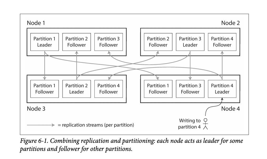Figure 6-1 in the book shows this leader / follower scheme for partitioning among multiple nodes.

• The goal in partitioning is to try and spread the data around as evenly as possible.
• If data is unevenly spread, it is called skewed.
• Skewed partitioning is less effective as some nodes work harder while others are sitting more idle.
• Partitions with higher than normal loads are called hot spots.
• One way to avoid hot-spotting is putting data on random nodes.
  • Problem with this is you won’t know where the data lives when running queries, so you have to query every node, which is not good.

Partitioning by Key Range

• Assign a continuous range of keys on a particular partition.
  • Just like old encyclopedias or even the rows of shelves in a library.
  • By doing this type of partitioning, your database can know which node to query for a specific key.
  • Partition boundaries can be determined manually or they can be determined by the database system.
  • Automatic partition is done by BigTable, HBase, RethinkDB, and MongoDB.
  • The partitions can keep the keys sorted which allow for fast lookups. Think back to the SSTables and LSM Trees.
• They used the example of using timestamps as the key for sensor data – ie YY-MM-DD-HH-MM.
• The problem with this is this can lead to hot-spotting on writes. All other nodes are sitting around doing nothing while the node with today’s partition is busy.
  • One way they mentioned you could avoid this hot-spotting is maybe you prefix the timestamp with the name of the sensor, which could balance writing to different nodes.
  • The downside to this is now if you wanted the data for all the sensors you’d have to issue separate range queries for each sensor to get that time range of data.
  • Some databases attempt to mitigate the downsides of hot-spotting. For example, Elastic has the ability specify an index lifecycle that can move data around based on the key. Take the sensor example for instance, new data comes in but the data is rarely old. Depending on the query patterns it may make sense to move older data to slower machines to save money as time marches on. Elastic uses a temperature analogy allowing you to specify policies for data that is hot, warm, cold, or frozen.

Partitioning by Hash of the Key

• To avoid the skew and hot-spot issues, many data stores use the key hashing for distributing the data.
• A good hashing function will take data and make it evenly distributed.
• Hashing algorithms for the sake of distribution do not need to be cryptographically strong.
  • Mongo uses MD5.
  • Cassandra uses Murmur3.
  • Voldemort uses Fowler-Noll-Vo.
  • Another interesting thing is not all programming languages have suitable hashing algorithms. Why? Because the hash will change for the same key. Java’s object.hashCode() and Ruby’s Object#hash were called out.
  • Partition boundaries can be set evenly or done pseudo-randomly, aka consistent hashing.
• Consistent hashing doesn’t work well for databases.
• While the hashing of keys buys you good distribution, you lose the ability to do range queries on known nodes, so now those range queries are run against all nodes.
• Some databases don’t even allow range queries on the primary keys, such as Riak, Couchbase, and Voldemort.
• Cassandra actually does a combination of keying strategies.
  • They use the first column of a compound key for hashing.
  • The other columns in the compound key are used for sorting the data.
    • This means you can’t do a range query over the first portion of a key, but if you specify a fixed key for the first column you can do a range query over the other columns in the compound key.
    • An example usage would be storing all posts on social media by the user id as the hashing column and the updated date as the additional column in the compound key, then you can quickly retrieve all posts by the user using a single partition.
• Hashing is used to help prevent hot-spots but there are situations where they can still occur.
  • Popular social media personality with millions of followers may cause unusual activity on a partition.
  • Most systems cannot automatically handle that type of skew.
  • In the case that something like this happens, it’s up to the application to try and “fix” the skew. One example provided in the book included appending a random 2 digit number to the key would spread that record out over 100 partitions.
  • Again, this is great for spreading out the writes, but now your reads will have to issue queries to 100 different partitions.
• Couple examples:
  • Sensor data: as new readings come in, users can view real-time data and pull reports of historical data,
  • Multi-tenant / SAAS platforms,
  • Giant e-commerce product catalog,
  • Social media platform users, such as Twitter and Facebook.

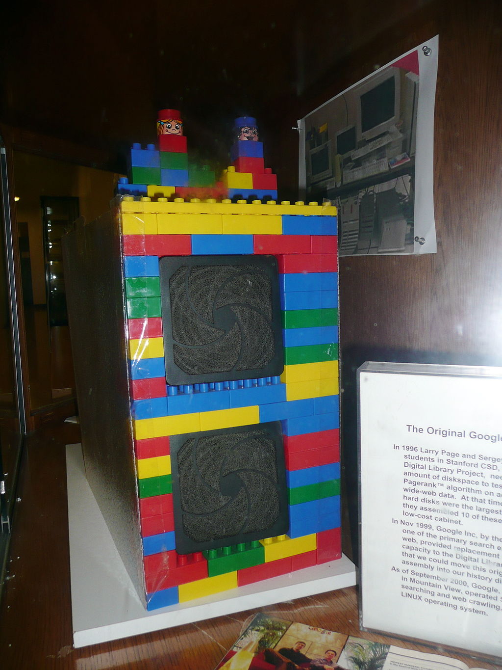The first Google computer at Stanford was housed in custom-made enclosures constructed from Mega Blocks. (Wikipedia)

Resources We Like

• Designing Data-Intensive Applications: The Big Ideas Behind Reliable, Scalable, and Maintainable Systems by Martin Kleppmann (Amazon)
• History of Google (Wikipedia)

Tip of the Week

• VS Code lets you open the search results in an editor instead of the side bar, making it easier to share your results or further refine them with something like regular expressions.
• Apple Magic Keyboard (for iPad Pro 12.9-inch – 5th Generation) is on sale on Amazon. Normally $349, now $242.99 on Amazon and Best Buy usually matches Amazon.(Amazon)
  • Compatible Devices:
    • iPad Pro 12.9-inch (5th generation),
    • iPad Pro 12.9-inch (4th generation),
    • iPad Pro 12.9-inch (3rd generation)
• Room EQ Wizard is free software for room acoustic, loudspeaker, and audio device measurements. (RoomEQWizard.com)